by

Mike McGuire

In conics I can floor peculiarities parabolous

(from the modern Major General's song)

E. C. Powell had a unique algorithmic approach to designing rod tapers. There were three types, the A taper, the B, and the C. The B taper was the simplest, just a straight line of constant slope. He set a tip dimension and the increase in dimension for every six inches. A typical increase he used was 8.7 thousandths for the six inches for the dimension of the strip. This is of course half the flat-to-flat dimension for a hex rod. In mathematical terms with a tip dimension y₀, and the increase in dimension per 6 inches, P, the dimension y at a point x along the rod is

The A and C tapers start with a B taper and are mirror images of each other with respect to the B taper. He set a small increment of say around 0.0004 inches. For an A taper at the first 6” station, the dimension was the B taper plus one increment. At the second it was the B taper plus two increments plus the increment of the first station for a total of three. At the third station it was the B taper plus three increments plus the previously added increments for a total of six and so on. If the increment is I, then at each station

                                                                     y₁ = y₀ + P + I,                                                              (2)

                                                                     y₂ = y₁ + P + 2I,                                                            (3)

                                                                     y₃ = y₂ + P + 3I,                                                            (4)

                                                                                 ...

                                                                      y_n = y_n-1 + P + nI,                                                       (5) or

                                                                      y_n = y₀ + nP + (1 + 2 + 3 + … + n) I.                          (6)

Now the sum of integers from 1 to n is n(n + 1) / 2, so

                                                                       y_n = y₀ + nP + [n(n + 1) / 2] I                                    (7)

With the C taper, the increment is subtracted so the equation looks like

                                                                       y_n = y₀ + nP - [n(n+1)/ 2] I.                                       (8)

Now n, the station number, varies with the distance from the tip x and the station spacing S so that

                                                                        n = x / S.                                                                    (9)

Putting this into the A taper equation, and considering x to vary continuously so we are not longer pinned to a station, we get

                                                                         y = (I / 2S² ) x² + [(P + I / 2) / S] x + y_0,                  (10)

and the C taper equation is

                                                                          y = - (I / 2S² ) x² + [(P - I / 2) / S] x + y_0.               (11)

Both of these equations have the form of a quadratic equation, which is to say the equation of a parabola,

                                                                           y = ax² + bx + c.                                                   (12)

Thus for an A taper

                                                                            a = (I / 2S² ),                                                         (13)

                                                                            b = [ (P + I / 2) / S ].                                             (14)

For a B taper

                                                                            a = 0,                                                                    (15)

                                                                            b = P.                                                                    (16)

For a C taper

                                                                            a = -(I / 2S² ),                                                       (17)

                                                                            b = [ (P - I / 2) / S ],                                              (18)

and

                                                                            c = y_0,                                                                   (19)

the tip dimension, in all cases.

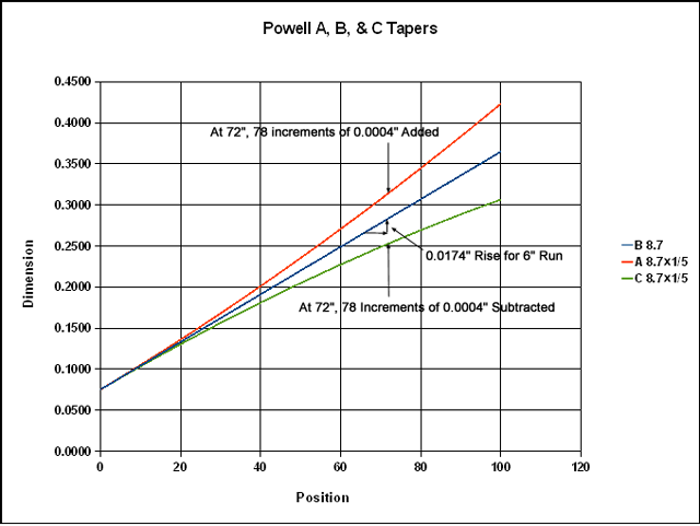
Powell spec'd his rods as A8.7x1/5 or C9x1/4. The 1/5 meant 1/5 of a thousandth or 0.0002 for the increment on a 6 inch station spacing. Below is what A8.7x1/5, B8.7, and C8.7x1/5 look like. In the plot, the dimensions are the flat-to-flat measurement rather than the strip measurements, so the parameters are doubled.

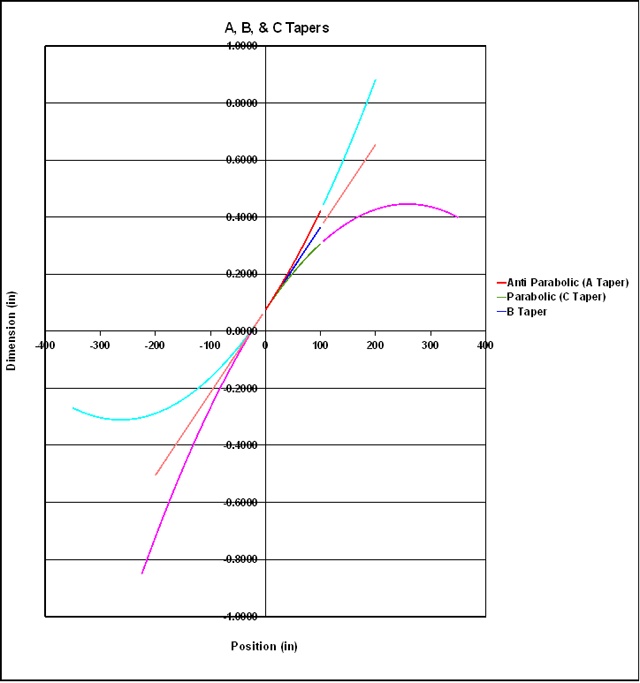
With more of the parabolas displayed, we can see where the parts used for rod tapers fit in.

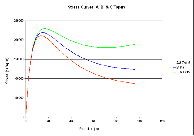
If we want to replicate a Powell taper for 5 inch forms, we need to multiply Powell's increment I, by (5/6)², and the slope P by 5/6. In theory there would be a further correction to P for the different increment, but it's negligibly small. Most of my information on the Powell tapers come from an article on them in Best of the Planing Form 2 by Ed Hartzell. In it he says that the A tapers varied from mild with an increment of 1/6 of a thousandth , to severe at 1/4 of a thousandth. However there was not much information about C tapers, although he did remark that he had heard of a C10x3/5, saying "anything is possible if you can cast well enought." Powell's own comments on his types of rods can be read at this link. I designed and made what I thought were A 8.7x1/5, B8.7, and C8.7x1/5 0.075 inch tip rods, 96” long—about 6 weights, and hollowed with Powell's scallop and dam style. Not having done the analysis above at the time, I had thought that multiplying the increment by 5/6 was sufficient to correct for 5 inch spacing rather than (5/6)². This put me pretty close to the “severe” level for the A taper, and indeed it was a real cannon. The B taper was pleasant as was the C taper, which was noticeably slower than the B, and mildly parabolic as shown by the dip in its stress curve. (in addition to actually being a parabola). In the sense usually meant in rodmaking one might call a A taper “anti-parabolic.”

Aside from Ed Hartzell's comment I have found nothing on C tapers, neither the parameters nor measured tapers, so I decided to try a little reverse engineering. Quite a number of tapers are available that are labeled “Parabolic”, notably the Paul Young Para series. There are nine different versions of of the Para 15 in the RodDNA database. I looked at them all. This is the first one, noted that it came by way of George Maurer. That taper is 

0	5	10	15	20	25	30	35	40	45	50
0.070	0.086	0.107	0.123	0.138	0.157	0.170	0.189	0.208	0.225	0.239

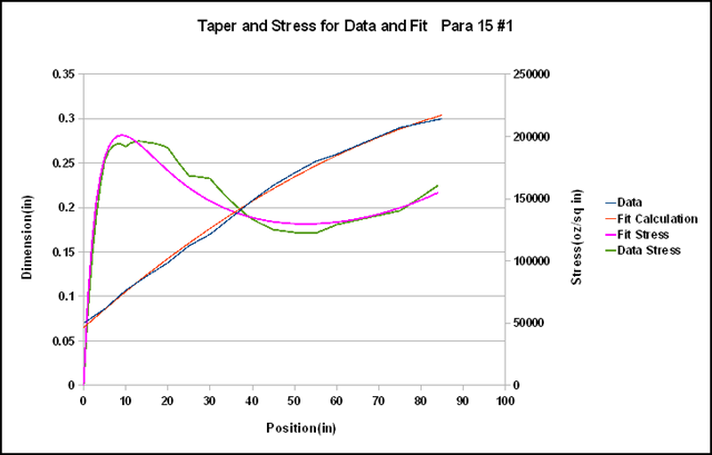
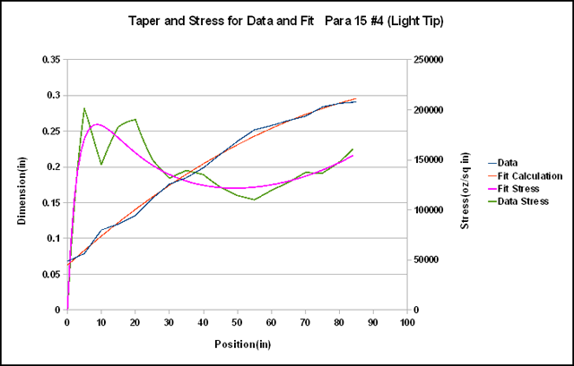
So I did a curve fit of a parabola to derive the a, b, and c parameters of the closest fitting parabolic curve out to 90” after which the taper doesn't change. Below is a plot of the data and the fit for a Para 15, along with the stress curves with 50' of 6 weight line. The fit seems remarkably close. The Powell parameters of the fit are P = 12.8, I = -0.00083. However, these are for a full flat-to-flat measure with 5” spacing, not 6”and a strip as Powell used. That I is for 5” spacing, not 6” and a strip as Powell used, so to put them in his terms, we divide by two and , so it would be about a C12.8x3/5.

To demonstrate this is not a fluke here is another version of the Para 15 with more variation but obviously following the parabolic trend.

The Powell parameters of this fit are P = 13.07, I = -0.00089, somewhat different from the first one. All of the Para series tapers had fits at least as good as the one above. It therefore seems possible, perhaps even likely, that Young started with actual parabolas when designing these rods and added his tweaks in the form of the small deviations we see. The spreadsheet I used to do these fits is available below for further exploration. I have made a rod with the “Powellized” version of the first taper and hollowed . I have found it quite pleasing as have others who have cast it. I also checked out some of the Pezon et Michel tapers that have parabolic in their names, and also found good fits there.

The kinks that appear in tapers and related stress curves are an artifact of plotting them as points 5” apart and connecting them with straight lines. In reality planing forms and Morgan Hand Mills function like rather large thick drawing splines, smoothing out the kinks . These can be modeled with cubic splines. This amounts to connecting the points with curves defined by cubic equations which have the form

                                                                   y = ax³ +bx² + cx + d.

The a, b, c, and d for each section are determined subject to the conditions that the curves join at the set points, their slopes at the set points are equal (first derivatives) , and the rates of change of the slopes at the set points are equal (second derivatives). This models the actual behavior of a real drawing spline. The details of how to do this can be found at this link. I did a spreadsheet which does this for an input taper. It calculates the splines and uses them to interpolates the points of the input taper at one inch intervals, and calculates the resulting stress curve. Below is the result for the Para 15 #4.

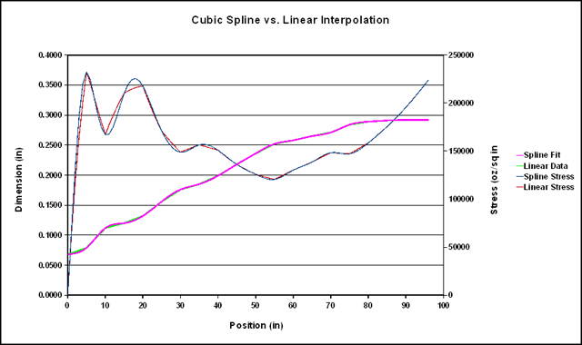
The effect on the taper curve is fairly subtle. In the plot the straight line taper is mostly covered up by the spline fit. In the numerical data for this the differences are mostly under 0.001” with a few near the tip becoming as large as 0.003”. The effect on the stress curve is noticeable. The structure is still there, but much smoother. This spreadsheet is also available.

Down loads:

ParabolicFit.xls

CubicSpline.xls

SpreadsheetInstructions.pdf