Dimension Compensation for Hollowing Bamboo Rods
by Mike McGuireI0
= aD04
where D0 is the flat to flat dimension and a is a constant that depends on the geometry of the cross section--hex, penta, quad etc. Assumed in all this is scallop and dam hollowing with minimal length dams. If we hollow to a wall thicknes t, the new moment I1 is the moment of a solid rod of dimension D1 less the moment of what is removed by hollowing.
where D0 is the flat to flat dimension and a is a constant that depends on the geometry of the cross section--hex, penta, quad etc. Assumed in all this is scallop and dam hollowing with minimal length dams. If we hollow to a wall thicknes t, the new moment I1 is the moment of a solid rod of dimension D1 less the moment of what is removed by hollowing.
I1
= a[ D14
- (D1 - 2t)4 ]
To maintain stiffness
we have to have
I1
= I0
D14 - (D1 - 2t)4 = D04
or
D14 - (D1 - 2t)4 = D04
The constant a divides out of the
equation. To get the correction, given t and D0
, we must solve for D1.
If we expand and rearrange this equation, we get
D13
- 3tD12
+ 4t2D1
- 2t3 - D04/8t = 0
This is a cubic equation in
D1,
that is it has the form
ax3 + bx2
+ cx + d = 0
where a = 1, b = -3t, c = 4t2,
and d = 2t3
- D04/8t.
As with quadratic equations, cubic equations can be solved with
formulas, but they are much more complicated.. As usual, Google is our
friend and if we ask it for a cubic solver, it comes up with several
choices. One that I like is at this link.
One calculates a,
b, c, and d,
puts them in, clicks the
enter button button and it will give you the
result.. Actually it will give you three results--the first of them is
the one we want. The other two are complex numbers which will also
satisfy the equation, but which don't apply here..From that page is a
link to another page which shows all the formulas involved in the
solution--not for the mathematically faint of heart.
Going through a whole taper, calculating a, b, c, and d is a lot of work with a lot of opportunity for error.To get by that I set this calculation up in a spread sheet so that I could calculate for a whole rod in one shot. It then occured to me that it would be interesting to look at the effects of hollowing on the Garrison stress curve of the rod, so I added this to the spread sheet. This required modification of some of the formulas to take account of the hollowing. I will describe the details of this below. From this point, it wasn't much of a leap think of using the stress curve of a solid rod to calcluate the dimensions of a hollowed rod. This is much the same as when one uses the stress curve to get dimensions of a new solid rod for casting a different weight of line, as is implemented in RodDNA and Hexrod. So this is part of the spread sheet now too. It is available for download below. The main difficulty was that another cubic equation turned up in going from the moment at a point on the rod to the dimension.
Here are some results. The rod is a Garrison 212 casting 50 feet of 6 wt line. The hollowing is fairly conservative, the butt third has a 0.070" wall, the middle third 0.060", and the tip third not hollowed. The results named "compensated" are the simple method where the moment of inertia is held constant as described above. Hollow output stress is when the rod is hollowed but no correction is done.
The differences from the solid rod are small where the hollowing starts, becoming larger toward the butt. The corrections from the stress curve are smaller than holding those from holding the moment of Inertia constant. The weights for the input solid rod and various amounts of hollowing are available from the stress curve calculations. These are the weights of just the bamboo. No hardware is included.
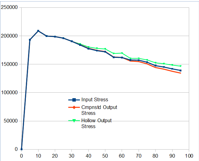
There is not a lot of difference between these curves with the conservative hollowing. The picture changes if we hollow more aggressively.
Since more correction is required it is not surprising to see larger dimension differences from the solid rod.
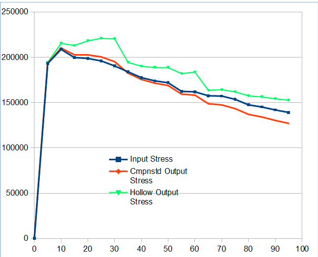
The stress curve (green) of the uncorrected hollowed rod is getting a bit wild here.
New version correcting errors as of 7/8/17
Solid2Hollow.xls
Going through a whole taper, calculating a, b, c, and d is a lot of work with a lot of opportunity for error.To get by that I set this calculation up in a spread sheet so that I could calculate for a whole rod in one shot. It then occured to me that it would be interesting to look at the effects of hollowing on the Garrison stress curve of the rod, so I added this to the spread sheet. This required modification of some of the formulas to take account of the hollowing. I will describe the details of this below. From this point, it wasn't much of a leap think of using the stress curve of a solid rod to calcluate the dimensions of a hollowed rod. This is much the same as when one uses the stress curve to get dimensions of a new solid rod for casting a different weight of line, as is implemented in RodDNA and Hexrod. So this is part of the spread sheet now too. It is available for download below. The main difficulty was that another cubic equation turned up in going from the moment at a point on the rod to the dimension.
Here are some results. The rod is a Garrison 212 casting 50 feet of 6 wt line. The hollowing is fairly conservative, the butt third has a 0.070" wall, the middle third 0.060", and the tip third not hollowed. The results named "compensated" are the simple method where the moment of inertia is held constant as described above. Hollow output stress is when the rod is hollowed but no correction is done.
| Position | | Input Dimension | Cmpnstd Output Dimension | Stress Crv Output Dimension | Input Stress | Cmpnstd Output Stress | Hollow Output Stress |
| 0 | 0.0720 | 0.0720 | 0.0720 | 0 | 0 | 0 | |
| 5 | 0.0840 | 0.0840 | 0.0840 | 193178 | 193178 | 193178 | |
| 10 | 0.1040 | 0.1040 | 0.1040 | 208755 | 208755 | 208755 | |
| 15 | 0.1220 | 0.1220 | 0.1220 | 199713 | 199713 | 199713 | |
| 20 | 0.1360 | 0.1360 | 0.1360 | 198724 | 198724 | 198724 | |
| 25 | 0.1490 | 0.1490 | 0.1490 | 195985 | 195985 | 195985 | |
| 30 | 0.1620 | 0.1620 | 0.1620 | 190457 | 190457 | 190457 | |
| 35 | 0.060 | 0.1750 | 0.1754 | 0.1756 | 183995 | 184434 | 185784 |
| 40 | 0.060 | 0.1880 | 0.1888 | 0.1891 | 177512 | 178094 | 180379 |
| 45 | 0.060 | 0.2000 | 0.2014 | 0.2016 | 174026 | 174602 | 177954 |
| 50 | 0.060 | 0.2120 | 0.2140 | 0.2142 | 171887 | 172347 | 176937 |
| 55 | 0.060 | 0.2280 | 0.2312 | 0.2314 | 162358 | 162777 | 168969 |
| 60 | 0.060 | 0.2400 | 0.2442 | 0.2443 | 161897 | 162016 | 169694� |
| 65 | 0.070 | 0.2540 | 0.2568 | 0.2557 | 157557 | 155689 | 160292 |
| 70 | 0.070 | 0.2660 | 0.2697 | 0.2682 | 157217 | 154755 | 160445 |
| 75 | 0.070 | 0.2800 | 0.2849 | 0.2829 | 153633 | 150706 | 157631 |
| 80 | 0.070 | 0.2960 | 0.3025 | 0.3000 | 147534 | 144284 | 152547 |
| 85 | 0.070 | 0.3100 | 0.3181 | 0.3150 | 145152 | 141401 | 150964 |
| 90 | 0.070 | 0.3250 | 0.3351 | 0.3312 | 141891 | 137676 | 148579 |
| 95 | 0.070 | 0.3400 | 0.3522 | 0.3475 | 139187 | 134461 | 146709 |
The differences from the solid rod are small where the hollowing starts, becoming larger toward the butt. The corrections from the stress curve are smaller than holding those from holding the moment of Inertia constant. The weights for the input solid rod and various amounts of hollowing are available from the stress curve calculations. These are the weights of just the bamboo. No hardware is included.
| Input Weight | Hollow Output Weight | Cmpnstd Output Weight | Stress Crv Output Weight |
| 2.67 | 2.08 | 2.12 | 2.11 |

There is not a lot of difference between these curves with the conservative hollowing. The picture changes if we hollow more aggressively.
| Position | | Input Dimension | Cmpnstd Output Dimension | Stress Crv Output Dimension | Input Stress | Cmpnstd Output Stress | Hollow Output Stress |
| 0 | 0.0720 | 0.0720 | 0.0720 | 0 | 0 | 0 | |
| 5 | 0.030 | 0.0840 | 0.0841 | 0.0842 | 193178 | 193469 | 194433 |
| 10 | 0.030 | 0.1040 | 0.1049 | 0.1052 | 208755 | 210247 | 215345 |
| 15 | 0.030 | 0.1220 | 0.1243 | 0.1249 | 199713 | 202598 | 213030 |
| 20 | 0.030 | 0.1360 | 0.1399 | 0.1409 | 198724 | 202581 | 218119 |
| 25 | 0.030 | 0.1490 | 0.1547 | 0.1560 | 195985 | 200449 | 220900 |
| 30 | 0.030 | 0.1620 | 0.1700 | 0.1715 | 190457 | 195216 | 220304 |
| 35 | 0.040 | 0.1750 | 0.1794 | 0.1786 | 183995 | 182483 | 194404 |
| 40 | 0.040 | 0.1880 | 0.1941 | 0.1930 | 177512 | 175559 | 190132 |
| 45 | 0.040 | 0.2000 | 0.2079 | 0.2063 | 174026 | 171519 | 188681 |
| 50 | 0.040 | 0.2120 | 0.2219 | 0.2199 | 171887 | 168839 | 188707 |
| 55 | 0.040 | 0.2280 | 0.2410 | 0.2386 | 162358 | 159355 | 182014 |
| 60 | 0.040 | 0.2400 | 0.2556 | 0.2524 | 161897 | 158272 | 183669 |
| 65 | 0.050 | 0.2540 | 0.2645 | 0.2577 | 157557 | 148787 | 163621 |
| 70 | 0.050 | 0.2660 | 0.2786 | 0.2706 | 157217 | 147513 | 164208 |
| 75 | 0.050 | 0.2800 | 0.2953 | 0.2859 | 153633 | 143378 | 161942 |
| 80 | 0.050 | 0.2960 | 0.3146 | 0.3038 | 147534 | 137075 | 157445 |
| 85 | 0.050 | 0.3100 | 0.3318 | 0.3193 | 145152 | 134094 | 156251 |
| 90 | 0.050 | 0.3250 | 0.3505 | 0.3362 | 141891 | 130354 | 154235 |
| 95 | 0.050 | 0.3400 | 0.3695 | 0.3531 | 139187 | 127109 | 152671 |
Since more correction is required it is not surprising to see larger dimension differences from the solid rod.
| Input Weight | Hollow Output Weight | Cmpnstd Output Weight | Stress Crv Output Weight |
| 2.67 | 1.58 | 1.69 | 1.58 |

The stress curve (green) of the uncorrected hollowed rod is getting a bit wild here.
The Spreadsheet
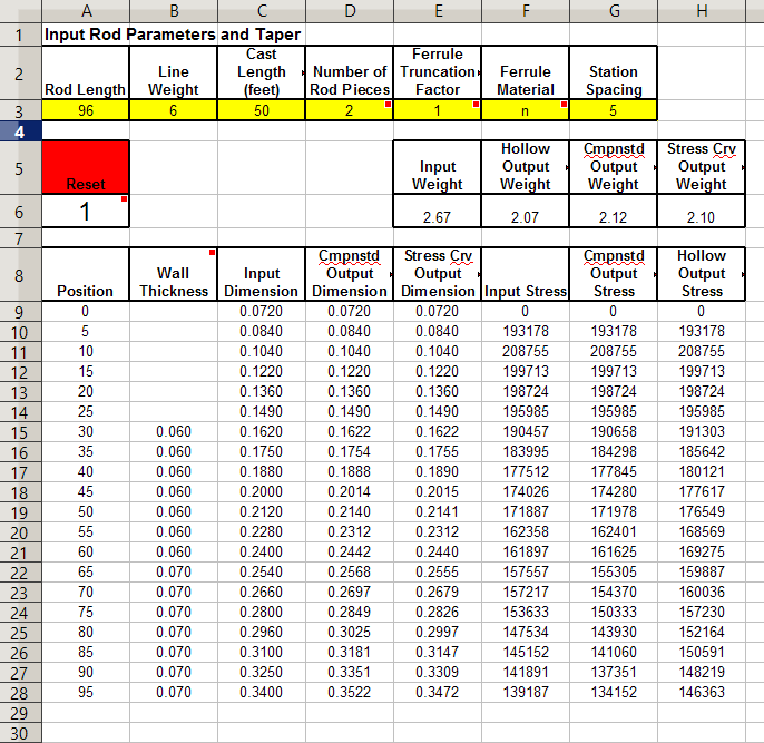
Below is a picture of part of the input/output sheet. To use it enter the rod parameters in the yellow line. The number of pieces can be 1, 2, 3, or 4. The truncation factor can be 1, 0.75 or 0.66. The station spacing can be whatever is the spacing of the input taper. The position values are automatically calculated from the length and the spacing. Leave the wall thickness blank where no hollowing is done. Otherwise don't make it greater than half the input dimension. The input taper can be copy/pasted from another app such as RodDNA or Hexrod. After all the input data is in place, enter 0 in the Reset box, push return, then enter 1, push return. This correctly initializes and then runs the iterative process that calculates the hollowed taper from the stress curve of the input taper. Depending on the previous contents of the sheet, garbage may appear as data is entered. The reset process should clean this up The graph of the stress curves appears to the right of what is seen below.The spreadsheet is protected This means only the input cells can be changed. This protects against accidental damage. There is no password on the protection. It can be removed at the users own risk if you want to tinker with it. It can be downloaded from the link below.New version correcting errors as of 7/8/17
Solid2Hollow.xls

Modifications of Garrison Stress Curve Formulas
For calculating a stress
curve the rod is divided into segments, typically the 5 inch segment of
the taper. The weight of each segement must be calculated. This is formula
III on page 251 of Garrrison.
W = 0.668 (h/3) [A + sqrt(A A1) + A1]
Wher A is the area of
the big end of the segment and A1
is the area of the small end,
h is the length,0.668
is the density of bamboo. This actually can be simplified a little by
noting that the area in terms of the flat to flat dimension D
A
= sqrt(3)/2 D2
then we have
W
= 0.668 [h / 2sqrt(3)] (D + DD1
+ D12)
where D is the dimension
of the big end and D1
the small end, sqrt
means square root. When we hollow, we must subtract off the weight of
what has been removed so we have W
= 0.668 [h / 2sqrt(3)] (D2 + DD1
+ D12-
d2 -dd1
- d12)
where d is the hollow dimension at the big end, d1 at the small end.
The location of the center of gravity C relative to its big end is required. This is formula IV on page 251.
again it can be simplified in terms of the dimension
When we hollow it becomes
Finally we have to deal with formula VI on page 258. This is the relation between moment at a point on a rod, the stress value, and the dimension. Garrison gives us.
Where M is the moment and f is the stress. If we solve this for the stress, we have
To deal with hollowing we have to go back to a more general equation for the relation.
Where I is the cross section moment of inertia. For a hexagonal cross section it is
if we put this into the general equation
having divided out a factor of D we get what Garrison gave us. If we hollow I becomes
where t is the wall thickness and the stress formula is
This is no problem for calculating the stress, we know M, D, and t. But if we know f, M, and t and want to find D, we have another cubic equation to solve. So rearranging the above equation, we get
The location of the center of gravity C relative to its big end is required. This is formula IV on page 251.
C = (h/4) [A + 2sqrt(AA1) +3A1] / [A + sqrt(AA1) + A1]
again it can be simplified in terms of the dimension
C = (h/4)(D2 +2DD1 + 3D12) / (D2 + DD1 + D12)
When we hollow it becomes
C = (h/4)(D2 +2DD1 + 3D12- d2 - 2dd1 - 3d12) /
(D2 + DD1 + D12- d2 -dd1 - d12)
(D2 + DD1 + D12- d2 -dd1 - d12)
Finally we have to deal with formula VI on page 258. This is the relation between moment at a point on a rod, the stress value, and the dimension. Garrison gives us.
D = (M / 0.120 f)1/3
Where M is the moment and f is the stress. If we solve this for the stress, we have
f = M / (0.120 D3)
To deal with hollowing we have to go back to a more general equation for the relation.
f = MD / 2I
Where I is the cross section moment of inertia. For a hexagonal cross section it is
I = [5 / 48 sqrt(3)] D4 = 0.06014 D4
if we put this into the general equation
f = M / (0.12028 D3)
having divided out a factor of D we get what Garrison gave us. If we hollow I becomes
I = 0.06014 [ D4 - (D - 2t)4]
where t is the wall thickness and the stress formula is
f = MD / { 0.12028 [ D4 - (D - 2t)4 ] }
This is no problem for calculating the stress, we know M, D, and t. But if we know f, M, and t and want to find D, we have another cubic equation to solve. So rearranging the above equation, we get
D3 - 3tD2 + [4t2 - M / (8 x 0.12028 f t) ] D - 2t3 = 0
When
we are getting a taper from the stress curve we have to solve this
equation for every station of the taper, multiple times as we converge
on the final value. This is built into the spreadsheet as is the
solution of the cubic for the simple conspensation for hollowing.